Large Vision Models (LVMs) are emerging tools for transferring cross-modal knowledge to time
series, but their potential for this domain is not yet fully understood. This work addresses
the gap by investigating LVMs for both high-level (classification) and low-level (forecasting)
time series tasks. Our aim is not only to assess whether LVMs can succeed, but also to reveal
why they succeed or fall short.
In these approaches, time series are imaged, i.e., transformed into certain
image representations, and then fed into an LVM to learn embeddings that can be probed for
downstream tasks. In this work, “LVM” is used to refer to image-pretrained vision models with
standalone vision backbones. Vision-language and multimodal foundation models are beyond the
scope of this work.
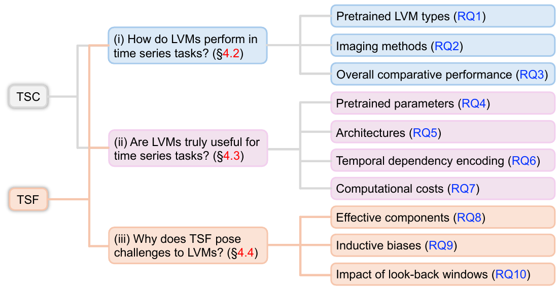
An overview of the structure of the experiments. “RQ” stands for research question.
Through a comparative benchmark covering four representative LVMs, eight imaging methods,
18 datasets, and 21 baselines, we identify the strengths and limitations of the foundational
LVMs, as well as effective strategies for adapting them to time series modeling. In a
nutshell, our conclusion is that pretrained LVMs prove versatile for time series
classification (TSC) – a task that relies on pattern comparison – but remain constrained for
time series forecasting (TSF), which requires precise numerical inference. Current
best-performing LVM-based forecasters, although effective, remain confined to specific types
of LVMs and imaging methods, exhibit biases toward forecasting periodic components in time
series, and struggle with long look-back windows.
Unlike prior works that question the adoption of Transformers and LLMs in this field, we take a
cautiously optimistic view, aiming to provide novel insights and practical caveats for
selecting and adapting LVMs to appropriate time series tasks in order to support future
developments. The experiments are organised as ten research questions (RQs) in three groups,
as shown alongside.
Setup
Image the series, then hand it to a vision model
This work does not aim to introduce new models. Instead, we assess LVMs’ innate ability for
time series analysis by keeping the main architecture intact while making a few necessary
modifications for cross-modal adaptation: (i) input alignment and (ii) task-specific
augmentation. The study involves two supervisedly pretrained LVMs, ViT and Swin, and two
self-supervisedly pretrained LVMs, MAE and SimMIM, along with eight widely used methods for
imaging time series.
Input alignment
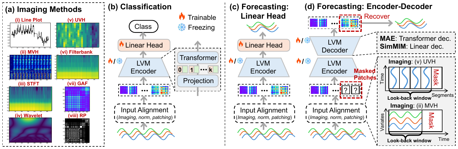
Line Plot draws a 2D image with the x-axis representing time steps and the y-axis representing
time-wise values. UVH (Univariate Heatmap) divides a univariate series into segments of length
L – where L is a period obtained using the Fast Fourier Transform – and stacks them into a 2D
image. MVH (Multivariate Heatmap) visualizes the matrix of a multivariate series, with the
x-axis representing time steps and the y-axis representing variates. STFT, Wavelet and
Filterbank transform the series into a spectrogram; GAF and RP produce square matrices with
both axes representing time. The imaged series is resized to the LVM’s pretraining input size
via bilinear interpolation, duplicated three times to form a grayscale image, and standardized
in the same manner as the LVMs standardize each pretraining image.
Task-specific augmentation
For the TSC task, we probe each LVM’s encoder: the classification layers of ViT and Swin, and
the reconstruction decoders of MAE and SimMIM, are replaced with a linear classification layer.
For the TSF task, we employ two frameworks from the literature. One trains a linear forecaster
on the concatenated CLS and patch embeddings and applies to ViT and Swin; the other uses LVM
reconstruction decoders for forecasting and applies to MAE and SimMIM – it applies a mask after
the look-back window portion of the image, then reconstructs the masked patches and recovers
forecasts from them. This requires input images to preserve time series values at the pixel
level, and among the eight imaging methods only MVH and UVH do.
Ablation models
To assess whether the LVM architecture is overly complex, we introduce two ablation models.
Both retain the projection layer in the LVM encoder but replace the Transformer with simpler
layers: the first replaces it with a linear layer, referred to as w/o-LVM; the second uses a
single randomly initialized multi-head attention layer, referred to as LVM2Attn.
(a) Different imaging methods, (b) LVM-based time series classification, (c) LVM with linear
head for forecasting, (d) LVM encoder-decoder for forecasting. In (a), MVH encodes multivariate
series, others encode univariate series. (b)(c) apply to all LVMs (ViT, Swin, MAE, SimMIM) in
this study; (d) applies to MAE and SimMIM with UVH/MVH images.
Performance
Versatile for classification, constrained for forecasting
What type of LVM best fits the TSC (TSF) task?
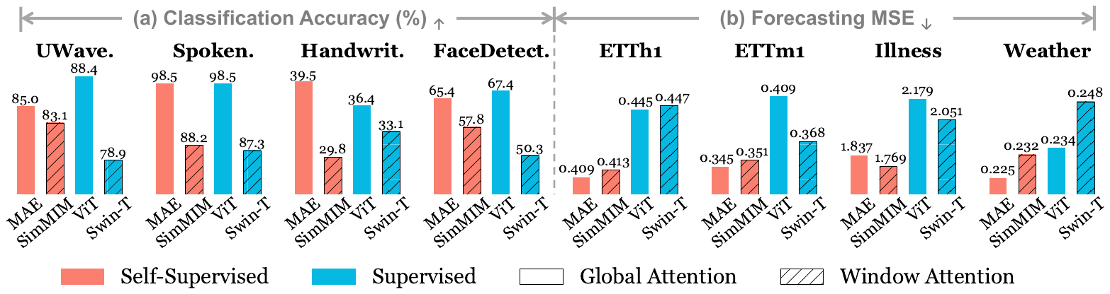
We observe that (1) supervised (semantic-level) LVMs and self-supervised (numerical-level) LVMs
achieve comparable classification accuracies, while (2) self-supervised LVMs substantially
outperform supervised LVMs in forecasting. Observation (2) can be attributed to the continuous
nature of both pixels and time series, which enables self-supervised LVMs to transfer their
capability of reconstructing masked pixels to predicting masked time series. SimMIM and Swin
underperform, likely because they employ a window-based local attention mechanism that
implicitly assumes translation invariance – an assumption that does not hold for imaged time
series, where different locations correspond to different time steps or frequencies.
Comparison of four LVMs on the TSC (accuracy, higher is better) and TSF (MSE, lower is better)
tasks. Two taxonomies of the LVMs: (1) supervised (ViT, Swin) vs. self-supervised (MAE,
SimMIM), and (2) global attention (ViT, MAE) vs. window-based attention (Swin, SimMIM).
Which imaging method best fits the TSC (TSF) task?
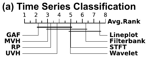
GAF performs best for classification, followed by MVH and RP, indicating their ability to
encode distinguishable temporal patterns. In contrast, Line Plot substantially underperforms
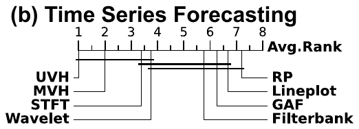
and therefore may be less suitable for this task. For forecasting, when combined with the
reconstruction framework, UVH achieves the best performance, followed by MVH. This suggests
their suitability for numerical-level tasks by leveraging the knowledge acquired by LVMs during
masked-pixel reconstruction in large-scale image-based pretraining.
Average ranks of the imaging methods in the TSC task. Lower ranks indicate better performance.
Average ranks of the imaging methods in the TSF task. Lower ranks indicate better performance.
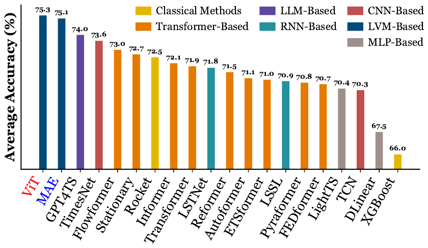
Model comparison on the TSC task. The results are average accuracy (%) over ten UEA datasets.
Can LVMs achieve SOTA performance?
Here ViT and MAE are selected as the best-performing supervised and self-supervised LVMs, each
configured with its best-performing imaging method – GAF for TSC and UVH for TSF. In
classification, both ViT and MAE outperform the baselines, suggesting both supervised and
self-supervised LVMs are effective for the high-level (semantic/pattern level) TSC task. In
forecasting, across the eight datasets and two metrics, MAE outperforms non-LVM baselines in
9/16 cases, while ViT does not show clear superiority over non-LVM baselines, which may be due
to its classification-based pretraining. The results suggest distinct behaviors of LVMs in TSF,
indicating that greater challenges may arise in low-level (numerical level) tasks.
Model comparison on the TSF task, averaged over forecasting horizons; lower MSE and MAE are
better. # Wins is the number of times each method performs best.
Ablations
Where the gains actually come from
This section aims to uncover whether the effectiveness of LVMs truly stems from their
pretrained parameters, architectures, and temporal modeling capabilities, and assesses their
computational costs. Unless otherwise noted, the best-performing LVM is used for each task:
ViT with GAF imaging for TSC and MAE with UVH imaging for TSF.
Are the pretrained parameters in LVMs useful?
For TSC, the “freezing all parameters” setting outperforms “training from scratch” in all
cases, suggesting that LVMs indeed transfer useful knowledge, and fine-tuning only the MLP and
normalization layers is the minimal effort required to achieve performance comparable to full
fine-tuning. For TSF, surprisingly, neither the “freezing all parameters” setting nor the
“fine-tuning all parameters” setting consistently outperforms “training from scratch”. In
contrast, fine-tuning only the normalization layers is generally better than
other training and fine-tuning strategies. This may be attributed to the low-level nature of
forecasting: since the model must predict numerical values directly, performance is strongly
influenced by normalization, whereas fine-tuning more parameters than necessary may lead to
overfitting.
How useful are LVM architectures?
Training LVMs from scratch does not consistently outperform the two simpler models, suggesting
that the architecture of LVMs alone may be overly complex for the available training data;
however, since training from scratch is generally no worse than the simpler models, the
overfitting issue does not appear to be severe. Moreover, the “freezing all parameters” setting
and all fine-tuning settings outperform the simpler models in TSC, while fine-tuning the
normalization layers consistently outperforms them in TSF. These results indicate that
LVM architectures are not overly complex when serving as containers of transferable
knowledge acquired through pretraining.
TSC reports accuracy (%, higher is better); TSF reports MSE (lower is better). The upper panel
compares fine-tuning strategies, the lower panel the two simpler ablation models.
Can LVMs capture temporal dependencies?
We perturb the temporal order in four ways: Sf-All randomly shuffles all time points; Sf-Half
randomly shuffles the first half; Ex-Half swaps the first and second halves; and Masking
randomly masks 50% of the time points. LVMs consistently exhibit performance drops under
temporal perturbations, and they are more vulnerable to these perturbations than the ablation
models. This suggests that LVMs likely make effective use of temporal patterns in time
series during inference.
Relative performance drops of the compared models under different temporal perturbations; the
accent marks the largest drop under each perturbation strategy.
What are the computational costs of LVMs?
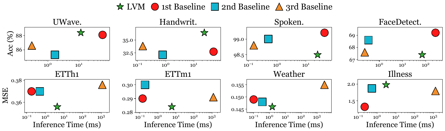
LVMs have a larger number of parameters than the baselines. On average, LVMs require 3x (16x)
the training time of the best TSC (TSF) baseline, primarily due to the larger number of
trainable parameters. For inference, LVMs are 4x faster than the best TSC baseline but 20x
slower than the best TSF baseline, due to both the increased model size and the additional
cost of transforming time series into images. Compared with the best baselines, LVMs trade a
relatively high computational overhead during inference for improved performance on many
datasets.
Inference time vs. performance of the compared methods in the TSC task (accuracy, higher is
better, the first row), and in the TSF task (MSE, lower is better, the second row).
Forecasting
Why forecasting is harder for vision models
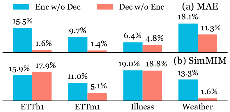
TSF performance drop (%) of (a) MAE and (b) SimMIM when initializing only the encoder with
pretrained parameters (blue) or only the decoder (red).
Which component of LVMs contributes more to TSF?
Usually, pretrained encoders are regarded as general feature extractors, whereas decoders are
often task-specific and re-trained for downstream tasks. However, the intuition appears to be
reversed when adapting LVMs to TSF. We compare two ablations: Enc w/o Dec, which fine-tunes the
pretrained encoder while re-training a randomly initialized decoder, and Dec w/o Enc, which
fine-tunes the pretrained decoder while re-training a randomly initialized encoder. Enc w/o Dec
exhibits a larger performance drop, suggesting that pretrained decoders contribute more
to TSF performance than pretrained encoders. This can be attributed to the fact that
LVM decoders are pretrained to reconstruct pixel values, making them naturally suited to the
numerical-level TSF task.
Notably, the decoder of SimMIM is merely a linear layer accounting for only 3.8% of the model
parameters, yet its contribution surpasses that of the substantially larger encoder. This
observation also helps explain the difficulty of adapting supervised LVMs to TSF, as they
typically lack pretrained decoders for numerical inference.
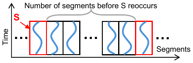
An illustration of UVH imaging: the number of segments before a segment S reoccurs.
Does the period-based UVH imaging method introduce any bias?
UVH stacks length-L segments of a univariate series into a 2D image, where L denotes the
period. We find that this method induces an inductive bias toward “forecasting
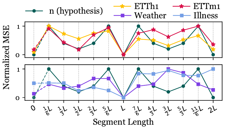
periods”. Evaluating MAE’s forecasting performance while varying the segment length
from L/6 to 2L, MAE achieves its best performance at L and 2L, suggesting that (1) the datasets
exhibit strong periodicity, and (2) MAE tends to forecast future values by “combining” past
periodic segments. When the segment length does not align with the underlying periods, MAE’s
forecasting accuracy deteriorates substantially.
TSF performance of MAE with respect to the segment length used in UVH imaging, with MSE
min-max normalized to [0, 1]. “n” (green) estimates TSF difficulty.
Under the UVH imaging framework, the forecasting difficulty is highly correlated with how
frequently a segment reoccurs, which can be quantified by the number of intervening segments
between two consecutive occurrences. If x has an exact period L and is divided into segments of
length (i/k)L, the smallest number of segments before a segment reoccurs is
n = k / GCD(i, k), where GCD denotes the greatest common divisor. The resulting “M”-shaped
curve of n aligns strongly with the MSEs on ETTh1 and ETTm1, supporting the estimation of TSF
difficulty and suggesting that MAE with UVH imaging has an inductive bias toward periodicity;
the MSEs on Weather and Illness align less well, likely due to their weaker periodicity. On
datasets of weak periodicity, MAE does not show a consistent advantage over the non-LVM
baseline, which further confirms the analysis and calls for diversifying benchmark datasets for
the TSF task.
Can LVMs make effective use of look-back windows?
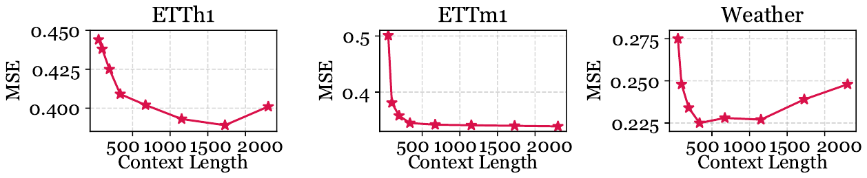
Intuitively, longer look-back windows can facilitate forecasting. MAE’s performance improves as
the look-back window increases up to certain steps (e.g., 500–1500), after which it plateaus or
declines. This behavior may stem from (1) the informativeness of a long look-back window, and
(2) the image transformation process: since pretrained LVMs operate on fixed-size images with a
limited number of pixels, they may be unable to capture all relevant information from
excessively long time series, and image pixels are not fully utilized by the UVH imaging method
to encode time-step information. Fortunately, contemporary LVMs can effectively handle
moderately long look-back windows, and a length of about a thousand time steps is sufficient
for many applications.
TSF performance (MSE) of MAE with varying look-back window (or context) lengths.
Outlook
Where the benchmark points next
Through extensive experiments across four representative types of LVMs, eight imaging methods,
18 datasets, and 21 baselines, we provide insights into whether image-pretrained LVMs are
effective for time series tasks, how to configure them for optimal performance, and what
challenges remain in LVM-based TSF. These insights can facilitate the adoption of LVMs for time
series analysis across research and applications.
Our benchmark study highlights several promising directions for future research:
(1) integrating different imaging methods to combine their distinct encoding capabilities;
(2) reducing inference latency in LVM-based TSF; (3) enhancing encoder utilization in LVM-based
TSF; (4) pretraining more effective decoders for LVM-based forecasters; (5) addressing or
harnessing the inductive bias of LVM-based forecasters; (6) improving pixel utilization for
encoding time series information in TSF; (7) developing encoders to learn multivariate
dependencies; (8) incorporating exogenous variates in TSF; and (9) disentangling the impact of
permuting variates when using the MVH imaging method. Moreover, a considerable portion of
current TSF benchmark datasets exhibit strong periodicity, which may lead to biased conclusions
about models with inductive biases similar to those of the UVH-imaging-based LVM forecasters;
diversifying benchmark datasets is therefore also an important future research direction.
Time series foundation models such as Chronos, Moirai, and LightGTS encode intra-modal
knowledge, i.e., knowledge acquired from large-scale time series pretraining, which is
complementary to the cross-modal (visual) knowledge encoded by LVMs. For example, a promising
future direction is to fine-tune image-pretrained LVMs on large-scale time series corpora,
thereby integrating both cross-modal and intra-modal knowledge to further enhance performance.
We hope this study complements existing research and lays the groundwork for future work on
multimodal, agentic time series analysis.
Additional backbones (DINOv2, MLCD, LaVin-DiT and the vision component of Qwen2-VL), LoRA
adaptation, variate permutations and a comparison with time series foundation models are in the
paper’s appendices.
Citation
Cite this work
BibTeX
@article{shen2026from,
  title   = {From Images to Signals: Are Image-Pretrained Vision Models Useful for Time Series Analysis?},
  author  = {ChengAo Shen and Hanghang Tong and Dongjin Song and Zhigang Deng and Qingsong Wen and Jingchao Ni},
  journal = {Transactions on Machine Learning Research},
  issn    = {2835-8856},
  year    = {2026},
  url     = {https://openreview.net/forum?id=aWVG2rN4OV},
  note    = {Featured Certification}
}