NeurIPS 2025 Long-Term Time Series Forecasting Large Vision Models Multi-Modal Views

DMMV

Multi-Modal View Enhanced Large Vision Models
for Long-Term Time Series Forecasting

ChengAo Shen1, Wenchao Yu2, Ziming Zhao1, Dongjin Song3, Wei Cheng2, Haifeng Chen2, Jingchao Ni1

1University of Houston   2NEC Laboratories America   3University of Connecticut

Paper arXiv Code BibTeX
Overview

One signal, several views of it

Time series, typically represented as numerical sequences, can also be transformed into images and texts, offering multi-modal views (MMVs) of the same underlying signal. These MMVs can reveal complementary patterns and enable the use of powerful pre-trained large models, such as large vision models (LVMs), for long-term time series forecasting (LTSF).

However, as we identified in this work, the state-of-the-art LVM-based forecaster poses an inductive bias towards “forecasting periods”. To harness this bias, we propose DMMV, a novel decomposition-based multi-modal view framework that leverages trend-seasonal decomposition and a novel backcast-residual based adaptive decomposition to integrate MMVs for LTSF.

Comparative evaluations against 14 SOTA models across diverse datasets show that DMMV outperforms single-view and existing multi-modal baselines, achieving the best mean squared error (MSE) on 6 out of 8 benchmark datasets.

Leveraging MMVs offers two key advantages: augmenting time series with alternative views can reveal patterns not evident in the original numerical data, and pre-trained large models can extract complex patterns specific to certain views, such as visual representations. DMMV integrates numerical and visual views in a compact architecture. We exclude the textual view due to its marginal gains in Time-VLM and recent doubts about the effectiveness and cost-efficiency of LLMs for LTSF.

Inductive bias

A forecaster that wants to repeat the period

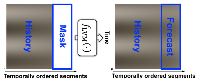
Masked autoencoder (MAE) is pre-trained self-supervisedly by reconstructing masked image patches using the ImageNet dataset. To adapt it to LTSF, VisionTS adopts a period-based imaging technique introduced by TimesNet: each length-T univariate series is segmented into ⌊T/P⌋ subsequences of length P, where P is set to be the period of the series, which can be obtained using the Fast Fourier Transform or from prior knowledge on sampling frequency. The subsequences are stacked to form a 2D image. After standard-deviation normalization, it is duplicated 3 times to form a gray image, followed by a bilinear interpolation to resize it to an image of size 224 × 224 × 3 to fit the input requirement of MAE. The forecast is achieved by reconstructing a right-appended masked area of that image, corresponding to the future horizon of the series.

Due to period-based imaging and the spatial consistency enforced during MAE's pixel inference, VisionTS exhibits a strong bias toward inter-period consistency, often overshadowing the global trend. The panels below illustrate VisionTS's forecasts on a synthetic sinusoidal time series with a period of 24. As the segment length P varies from 24 to 48, forecasts alternate between accurate and inaccurate as P shifts from 1×period to 2×period, highlighting a strong inductive bias toward periodicity. Notably, the forecasts aren't mere repetitions — the decreasing intra-period amplitude indicates that LVMs can still capture local trends within each period.

Forecasts of an LVM forecaster on a synthetic sinusoid under four different segment lengths.
An illustration of an LVM forecaster's inductive bias. The time series has a period of 24. The vertical dashed lines mark the segment points. The example indicates a bias towards segment lengths that are multiples of the period in (a) and (d) over other segment lengths in (b) and (c).

The function of the synthetic time series is x(t) = A(t) · sin(2πt / P), where the period P is set to 24 and the amplitude function A(t) decreases linearly over time. The forecasts are more accurate when the segment length is a multiple of the period (e.g., 24, 48) than other values. In the table below, the fluctuations in MSEs and MAEs across different segment lengths other than 24 and 48 support the findings of the inductive bias toward “forecasting periods”.

Forecasting performance of an LVM with respect to varying segment length on the synthetic dataset. Lower MSE and MAE are better.

Method

Two forecasters, two ways to split the signal

Motivated by this observation, we design the DMMV framework to leverage the inductive bias of LVMs while addressing their limitations. Specifically, the visual forecaster — the LVM — focuses on capturing periodic patterns from the visual view, while the numerical forecaster models global trends from the numerical view, resulting in more balanced forecasting.

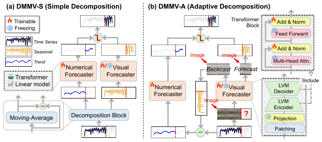
DMMV-S simple decomposition. It adopts a simple moving-average decomposition, which explicitly decomposes an input time series into a trend part and a seasonal (or periodic) part, reflecting the long-term progression and the seasonality of the series, respectively. Moving-average uses a kernel — a sliding window — of length 2⌊P/2⌋ + 1 to extract the component with frequency lower than the series' sampling frequency, highlighting the global trend; the residual component is the seasonal part. The visual forecaster transforms the seasonal input into a 224 × 224 × 3 image and outputs the forecast for the seasonal component.

The numerical forecaster rather than imposing a specialized inductive bias, we adopt a general-purpose architecture capable of capturing long-term dependencies. We investigate the feasibility of two options and leave other explorations as a future work: a simple linear model motivated by the proven effectiveness of linear methods in LTSF, and a Transformer-based model inspired by PatchTST, which segments the trend into N length-L patches, projects them to embeddings with a learnable positional encoding, and passes the Transformer output through flatten and linear operators to achieve the forecast for the trend part.

Gated late fusion finally, the seasonal and trend forecasts are merged to produce the overall forecast for the variate. In particular, instead of using the regular summation-based merge, we design an adaptive merge function with a light-weight gate g = sigmoid(wg) ∈ [0, 1], where wg is a learnable scalar parameter. DMMV employs late fusion via this gating mechanism, as intermediate fusion — at the embedding level, say — underutilizes MAE's decoder, which plays a crucial role in pixel prediction.

DMMV-A adaptive decomposition. One limitation of DMMV-S is the explicit trend-seasonal decomposition placed on the input, which will enforce the numerical and visual forecasters to fit pre-defined components extracted by a certain kernel size. This is not flexible and may not fully leverage LVMs' potential. Unlike DMMV-S, DMMV-A implicitly decomposes the input into trend and seasonal components tailored to the strengths of the numerical and visual forecasters, respectively. This is achieved via a backcast-residual mechanism that leverages LVMs' bias toward periodic patterns. The input is first transformed into an image using period-based imaging. Before forecasting, the visual forecaster is used to backcast the look-back window by reconstructing masked segments of that image.

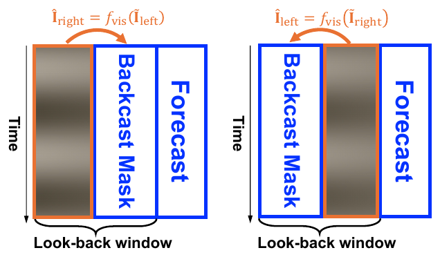
BCMask an effective masking strategy must enable full-window reconstruction, align with the forecasting setup, and minimize the usage of the visual forecaster to avoid computational overhead. To meet these criteria, we propose an efficient BackCast-Masking (BCMask) strategy, which applies two passes: masking and reconstructing the left and right halves of the image, respectively. BCMask satisfies all three criteria: it enables full reconstruction of the image; it uses contiguous segments to predict adjacent segments, mirroring the forecasting process; and it minimizes the use of the visual forecaster — only two passes are needed, as some unmasked regions of the image are required for prediction and must later be masked to complete the full reconstruction.

The residual is the trend notably, the backcast image is biased toward the periodic patterns in the input image. After de-normalization and reverse transformation, a backcast time series is recovered, reflecting the periodic component in the input; the residual — input minus backcast — therefore emphasizes the trend. We feed this residual into the numerical forecaster to produce the trend forecast, while the visual forecaster predicts from the input image, likely yielding the forecast of the seasonal component; the two are fused via the same gating mechanism. Unlike the backcast in N-BEATS — designed merely to extract predictive errors — our approach is specifically tailored to exploit LVMs' bias toward periodic patterns, making it fundamentally different.

Optimization DMMV is trained by minimizing the MSE between the forecast and the ground truth. The numerical forecaster is trained from scratch, while the visual forecaster uses pre-trained LVM weights with partial fine-tuning. We find that fine-tuning only the normalization layers yields the best performance. For the choice of LVM, we tested MAE and SimMIM, both self-supervisedly pre-trained; MAE performs better and is set as the default. Training begins with the visual forecaster frozen while the numerical forecaster is trained for a number of epochs, around 30. Then the norm layers of the visual forecaster are unfrozen and fine-tuned jointly with the numerical forecaster until convergence or early stopping.

An illustration of an LVM forecaster reconstructing a right-appended masked area.
An illustration of an LVM forecaster.
An illustration of BCMask, masking and reconstructing the left and right halves of the image.
An illustration of BCMask.
An overview of the DMMV framework, showing the simple-decomposition and adaptive-decomposition variants.
An overview of the DMMV framework. DMMV-S uses moving-average to extract trend and seasonal components. DMMV-A uses a backcast-residual decomposition to automatically learn trend and seasonal components. In DMMV-A, the gray blocks are gray-scale images; “?” marks masks.
Results

Best MSE on 6 of 8 benchmark datasets

We adopt 8 widely used multivariate benchmarks: ETT — ETTh1, ETTh2, ETTm1, ETTm2 — together with Weather, Illness, Traffic and Electricity. Following standard protocols, we split the datasets chronologically into training/validation/test sets using a 60%/20%/20% ratio for ETT and 70%/10%/20% for the others. The prediction horizon is set to {24, 36, 48, 60} for Illness and {96, 192, 336, 720} for the remaining datasets. By default, the look-back window is 336. We use Mean Squared Error and Mean Absolute Error to evaluate the LTSF performance of the compared methods.

The table below summarizes the LTSF performance of 10 representative methods across four categories: MMV-based, visual-view-based, language-view-based, and numerical-view-based approaches. Time-VLM's results on the Illness dataset are not reported in its paper and its code is unavailable at the time of this experiment, thus are marked by “—”. For DMMV, the stronger variant, DMMV-A, is reported.

Several key insights emerge: MMV and visual-view methods generally outperform language-view methods, underscoring the effectiveness of LVMs, particularly when integrated within MMV frameworks; numerical-view models such as PatchTST and CycleNet remain competitive, especially on datasets where VisionTS underperforms — ETTm2 and Electricity — highlighting their potential to complement visual models; the strong results of CycleNet, a lightweight model with learnable decomposition, demonstrate the value of combining simplicity with structure in LTSF; notably, DMMV-A, which unifies visual and numerical views through a novel adaptive decomposition, outperforms the baselines in most cases, achieving 43 first-places and confirming its effectiveness; and lastly, while VisionTS performs well on highly periodic datasets such as ETTh1, ETTm1 and Traffic due to MAE's inductive bias toward periodicity, DMMV-A alleviates this bias, resulting in more generalizable forecasts.

Dataset
Metric

Lower MSE and MAE are better. Views — Multi-Modal: DMMV-A, Time-VLM; Visual: VisionTS; Language: GPT4TS, Time-LLM; Numerical: PatchTST, CycleNet, TimesNet, DLinear, FEDformer. “# Wins” counts first places over all 8 datasets, all prediction horizons and the average rows. As we use the standard evaluation protocol, we collect baseline results from prior works; VisionTS is re-run with a look-back window of 336, and CycleNet is run on the Illness dataset with its official code.

Critical difference diagrams of the average MSE and MAE rank of all 16 compared methods.
Critical difference diagrams on the average rank of all 16 compared methods in terms of MSE and MAE over all benchmark datasets. The lower rank, to the left of the scale, is better. DMMV-S ranks 4.5/16 in MSE and 7.1/16 in MAE, underscoring the benefit of the adaptive decomposition used in DMMV-A; DMMV-S's comparable ranks to CycleNet indicate that even with a simpler, fixed decomposition, DMMV-S exhibits an ability that a strong SOTA model with learnable decomposition has.
Analysis

Decoder, fusion, mask, training and decomposition all matter

We validate the design of DMMV-A through ablation studies on four datasets: (a) replaces the linear model in the numerical forecaster with a PatchTST-style Transformer; (b) swaps MAE with SimMIM as the visual forecaster; (c) replaces the gating fusion with a simple sum; (d) removes BCMask, performing backcasting and forecasting on the full, unmasked look-back window; (e) substitutes BCMask with random masking; (f) freezes the entire visual forecaster instead of fine-tuning norm layers; and (g) removes the backcast-residual mechanism, feeding both forecasters the same input and merging their outputs via gating.

In (a), replacing the linear numerical forecaster with a Transformer slightly degrades performance, likely due to the increased difficulty of jointly training a Transformer with LVMs. In (b), MAE outperforms SimMIM as the visual forecaster, likely due to its ViT-based reconstruction decoder being better suited for pixel-level tasks like LTSF than SimMIM's linear decoder, while both models share similar encoder architectures. In (c), gate-based fusion outperforms simple summation, highlighting its adaptability to the distinct outputs of the two forecasters. (d) and (e) underscore the importance of BCMask: removing it recovers the full look-back window as the backcasted seasonal component, diminishing the trend signal and weakening the numerical forecaster, while random masking performs slightly worse due to poorer periodic pattern extraction, which leads to many fluctuations. In (f), fine-tuning only the norm layers significantly improves performance over freezing, confirming the benefit of coordinated learning between forecasters. Finally, (g) shows that removing the backcast-residual mechanism causes a major performance drop, affirming its role in effective decomposition.

MSE and MAE are averaged over different prediction lengths; lower is better. Improvement of each ablation is relative to DMMV-A, where a positive value is better.

Where the gate puts its weight

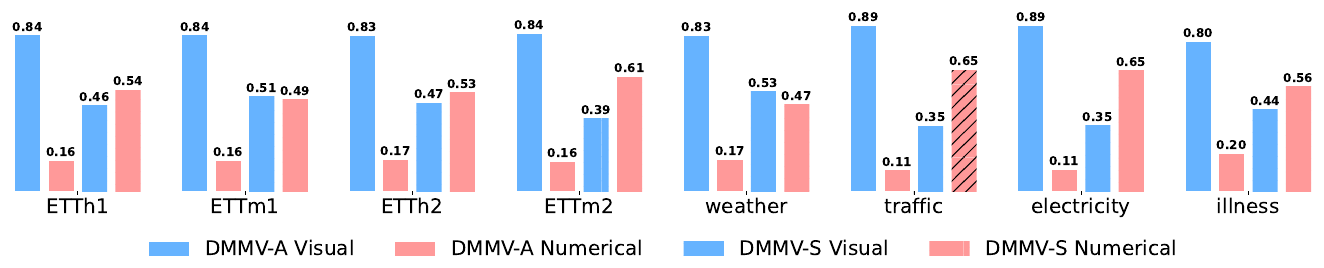
A key advantage of the gate-based fusion is its interpretability. The chart below presents average gate weights across datasets: DMMV-A consistently places more weight on the visual forecaster, while DMMV-S tends to balance both forecasters but leans toward the numerical one. In DMMV-A, these weights are learned based on forecasting performance, emphasizing the visual forecaster's importance. Notably, although the numerical forecaster receives less weight, it remains essential — as evidenced by DMMV-A outperforming the visual-only baseline VisionTS in the table above. In contrast, DMMV-S's weights are limited by its fixed moving-average decomposition, leading to a non-adaptive and suboptimal allocation of forecasting roles.

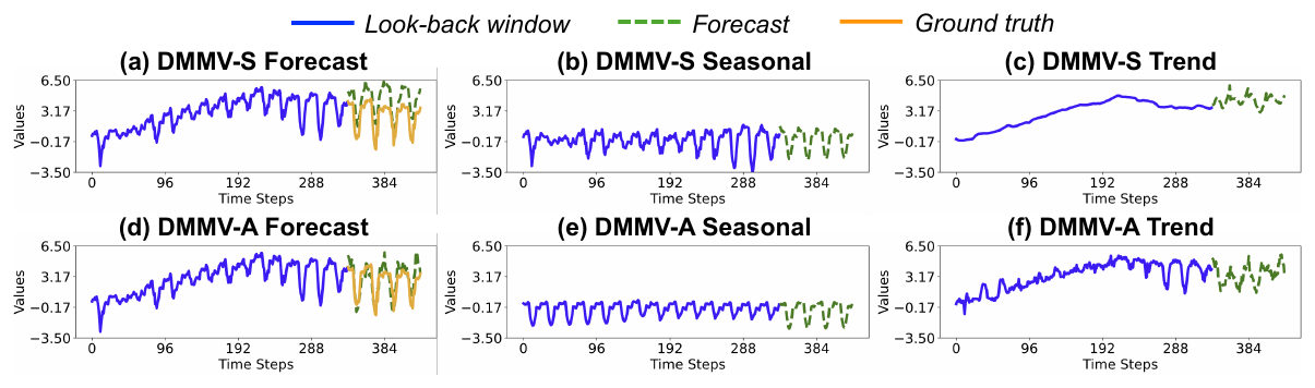
The example below provides decompositions by DMMV-S and DMMV-A. DMMV-A produces a smooth, clearly periodic component — consistent with expectations — and a trend component with some noises. In contrast, DMMV-S's moving-average yields a smoother trend by absorbing fluctuations, pushing noise into the seasonal component. This makes forecasting harder for the visual forecaster, which is more sensitive to fluctuations than the numerical one, resulting in its lower gate weights. Since periodic patterns are crucial for long-term forecasting, the clearer period separation in DMMV-A leads to forecasts that better match the ground truth.

Bar chart comparing DMMV-S and DMMV-A gate weights on the visual and numerical forecasters.
Comparing DMMV-S and DMMV-A with respect to gate weights on visual and numerical forecasters.
Forecasts, seasonal components and trend components of DMMV-S and DMMV-A on the same ETTh1 example.
The decompositions of DMMV-S and DMMV-A on the same example in ETTh1: (a) and (d) input time series and forecasts, (b) and (e) seasonal component, (c) and (f) trend component.

The impact of the look-back window

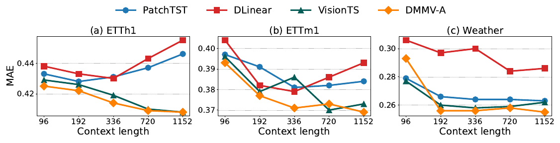
The plots below compare DMMV-A with a visual forecaster, VisionTS, and two numerical forecasters, PatchTST and DLinear, which can serve as its single-view ablations. The Illness dataset is excluded due to its short time series, 966 time steps in total. Using the MAE metric, we observe that DMMV-A and VisionTS benefit from longer look-back windows, while PatchTST and DLinear degrade beyond a length of 336. Notably, DMMV-A outperforms VisionTS at length 1152, highlighting the advantage of explicitly modeling global trends.

Average MAE of PatchTST, DLinear, VisionTS and DMMV-A under varying context lengths.
Average MAE comparison with varying look-back window, or context, lengths.
Citation

Cite this work

BibTeX
@inproceedings{shen2025dmmv,
  title     = {Multi-Modal View Enhanced Large Vision Models for Long-Term Time Series Forecasting},
  author    = {Shen, ChengAo and Yu, Wenchao and Zhao, Ziming and Song, Dongjin and Cheng, Wei and Chen, Haifeng and Ni, Jingchao},
  booktitle = {Advances in Neural Information Processing Systems},
  year      = {2025}
}